Portfolio Optimization with Genetic Algorithm

Portfolio Optimisation Using a Genetic Algorithm

Portfolio optimisation is one of the most interesting fields of study in financial mathematics. Many scientists have studied a lot of analytical and numerical methods to build the best investment portfolio according to a defined set of assets.

In this article, I’ll introduce a method to optimize a portfolio by using a numerical technique based on genetic algorithms. The power of genetic algorithms makes it possible to find the optimal portfolio even when the objective function isn’t smooth or differentiable. This heuristic search algorithm follows the darwinian theory of natural selection to discover optimal solutions among viable candidates. This is done by passing down the characteristics of “fit” candidates down to the succeeding generations allowing the determination of better fitness-scored solutions.

Portfolio Composition

Given we have N financial asset we want to invest in. These can be made up of bonds, ETFs, diversified funds and stock. Each being made up of historical returns that are the price relative difference from on period to another.

The return of the i -th asset between period t and period t-1 is defined as:

\[p_{i}(t) = \frac{\text{Price}_{i}(t)-\text{Price}_{i}(t-1)}{\text{Price}_{i}(t-1)}\]

With this the weighted portfolio return at a time t is then:

\[P(t)= \displaystyle\sum\limits_{i=1}^{N}x_{i}\cdot p_i(t)\]

The weighted return is given as a fraction of the capital allocated to each asset. The goal will be to determine the optimal value of weights that will maximize our objective function with respect to some constraints which are:

\[\displaystyle\sum\limits_{i=1}^{N}x_{i}=1 \quad 0 \leq x_{i}\leq 1\]

Objective function

A useful objective function for portfolio optimization is the Sharpe Ratio, defined as:

\[\text{Portfolio Sharpe} = \frac{E(P)}{\sqrt{Var(P)}}\]

Where E(P) is the expected return of the portfolio, Var(p) is the variance. The overall aim is to determine a portfolio whose returns are stable around the mean. Thus it is not the highest return that is sought, but the highest stability of portfolio.

Penalty Function method

Using the penalty function method, the problem is simplified by transforming it into an unconstrained optimisation problem. To do this, we create a new function that penalizes all points in the function domain that do no satisfy the constraints.

The inequality constraints can be written in the following manner:

\[x_{i} \leq 1 \Rightarrow [\text{max}(0,x_{i}-1)]^2\] \[x_{i} \geq 0 \Rightarrow [\text{max}(0,-x_{i})]^2\]

The summation constraint is an equality constraint which can easily be written as a penalty function.

\[f(x) - d = 0 \Rightarrow [f(x) -d]^2\]

So the sum equality constraint becomes:

\[\displaystyle\sum\limits_{i=1}^{N}= 1 \Rightarrow \Big( \displaystyle\sum\limits_{i=1}^{N} - 1 \Big)^2\]

Sharpe objective function

The terms are combined as follows:

\(-\text{Sharpe}({x_{i})}+ 100 \Big[ \Big( \displaystyle\sum\limits_{i=1}^{N} x_{i}-1 \Big)^{2} +\displaystyle\sum\limits_{i=1}^{N} \text{max} (0, x_{i}-1))^{2}+ \text{max} (0, -x_{i}))^{2}\Big]\) The penalty are multiplied by a factor of 100 to enhance the optimization process.

R Code Implementation.

The R implementation can be found in my github repository for Portfolio Optimization with GA.

Collect Data of Assets Returns

For this demonstration we have collected the historical data of the following assets:

Tesla
Amazon
Apple
Sibanye Stillwater
Gold Fields Limited
Sonos

The data is obtained from Yahoo Finance

## Optimisation via Genetic Algorithm

R has a general purpose Genetic algorithm packaged called “GA”. the following is an excerpt of its implementation in R.

{r}

library("GA")
ga_res = ga(
      # Tell the genetic algorithm that the 
      # weights are real variables
      type="real-valued", 
      
      # "ga" function performs maximization, so we must
      # multiply the objective function by -1
      function(x){-obj(x)}, 
      
      # x_i >= 0
      lower = rep(0,ncol(asset_returns)), 
      
      # x_i <= 1
      upper = rep(1,ncol(asset_returns)), 
      
      # Maximum number of iterations 
      maxiter = 50000, 
      
      # If the maximum fitness remains the same for 50
      # consecutive transactions, stop the algorithm
      run=50, 
      
      keepBest = TRUE,
      
      # Exploit multi-core properties of your CPU
      parallel=TRUE,
      
      # We want to see the partial results of the process
      # while it performs
      monitor=TRUE,
      
      # Seed useful for replicating the results
      seed=1
)

Optimisation Results

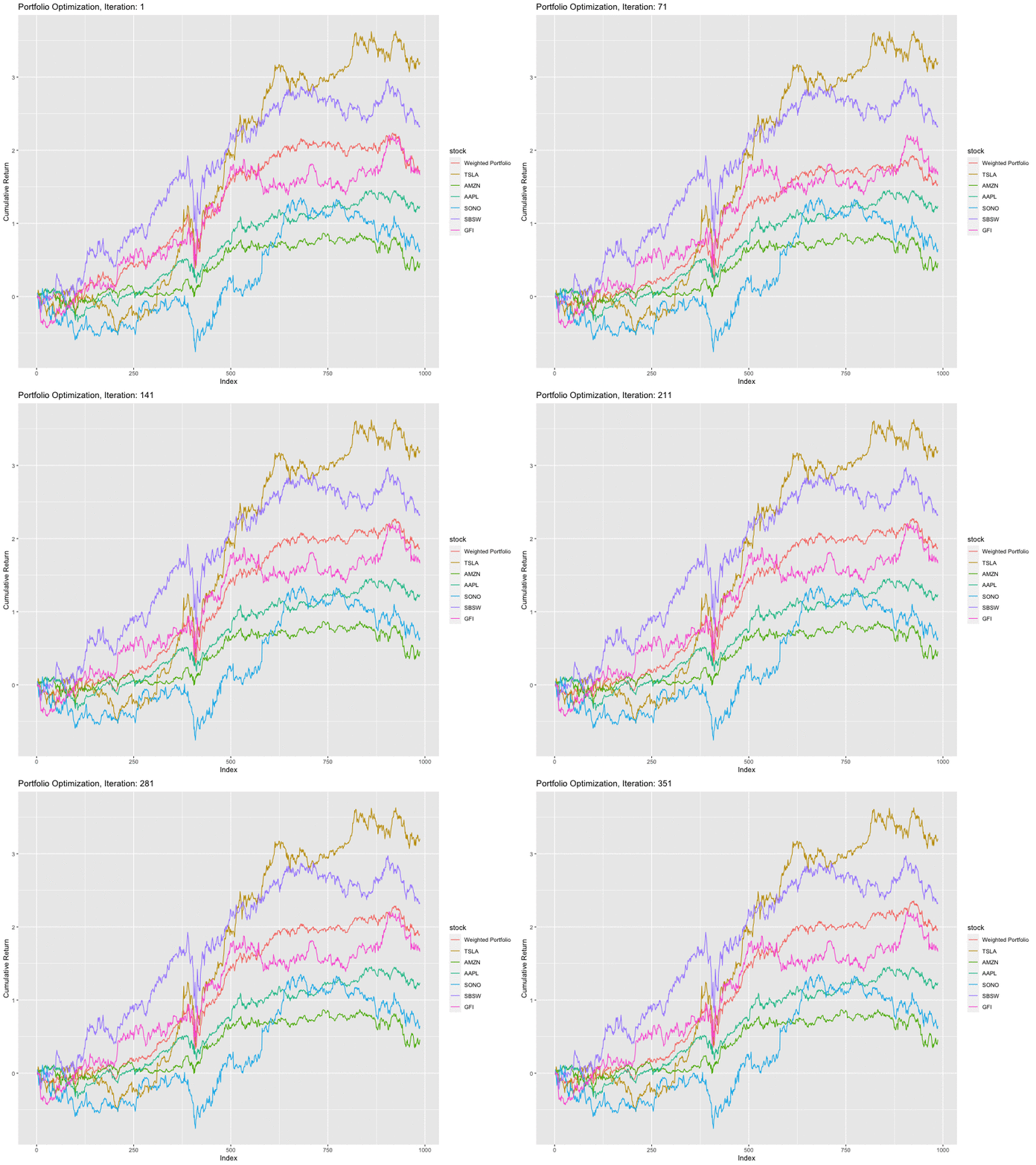
The final portfolio composition generated by genetic algorithm is as follows:

Tesla (29.1%), Amazon (7.1%), Apple (18.7%), Sono (8.9%), Sibanye (17.3%), Gold Fields (18.9%).

output

As you can see, the portfolio return (Orange line) is the most stable curve, although it’s not the best performing one (Apple and Sibanye performing better).

explicity_my3

It can be observed that with each iteration, the shape of the weighted portfolio slowly becomes less volatile. This has been merely a high level introduction, many additions can be made to suit the problem at hand and achieve better results. This can be done by employing a deterministic optimisation algorithm to further fine tune the results and improve precision.

← Previous Post Next Post →